
Before estimating the endurance on a single charge, we have to understand the normal use case to tune the radio parameters for minimizing power consumption. In this post, we will see some of those parameters, how they impact power consumption and how does one trade-off between them.
Power Measurement
During a BLE transaction radio circuitry is on, otherwise, it is off. During the radio-off period, the CPU core may be asleep or it might be processing some data. While asleep, the current consumption is very low (typically few uA), and when active during a BLE transaction the current consumption goes beyond a few mA because the radio circuitry consumes additional power in contrast with the CPU core.
The current consumption varies with time, in orders of magnitude, such amount of variation is harder to measure by a handheld Digital Multimeter. By using an oscilloscope with a current probe it’s easier to visualize current consumption over a period of time. The following parameters are useful when measuring current with an oscilloscope. For this test, we chose to use the nRF’s Power Profiling kit, which measures and displays the current waveform.
Average Current Consumption: It is the average current consumption over a given period of time.
Peak Current Consumption: It is the maximum current consumption observed during a given period of time.
We used the following setup for this exercise:
- Hardware:
- NRF52840 DK, PCA10056, v1.0.0
- nRF Power Profiler Kit, PCA63511, v1.1.0
- Software:
- nRF5-SDK, v17.0.2
- SoftDevice S140, v7.2.0
Parameters for Optimizing
The BLE Specification describes that “The physical channel is sub-divided into time units known as events. Data is transmitted between LE devices in packets that are positioned in these events. There are two types of events: Advertising and Connection events.” – Vol 1, Part A, Section 1.2.
These events periodically occur at a fixed interval. Between these periodic events, the CPU core is put to sleep until the start of the next event. During sleep, the power consumption is lowest, and during the event period, the power consumption reaches peak (maximum) value due to the Radio circuitry and CPU core being active. These events may timeout after a predefined duration or usually by disconnection event.
The specification allows us to tune Advertising & Connection intervals within a specified limit and it also aids the trade-off between Datarates and Power consumption.
Advertising Parameters
1. Advertising Interval
It is the time interval between two consecutive advertising events. During the advertising event, the radio is turned on to transmit an advertising packet, otherwise, the CPU core is asleep and the radio turned off between the advertising events. For example, with an advertising interval of 100ms, 10 advertising events occur within a period of 1 second. The radio is turned on 10 times. For shorter intervals, the radio is turned on more frequently consuming more power than it would if the advertising interval was 100ms. Similarly, for higher intervals, the radio is turned on less frequently consuming lesser power than it would if the advertising interval was 100ms.
Specification Limit: 20ms to 10.24s
The table below summarizes the measured current consumption at various advertising intervals. Followed by an image which is a series of snapshots from nRF’s Power Profiles tool taken during the measurement.
| Advertising Interval in ms | Avg. Current in mA | Peak Current in mA |
| 20 | 1.34 | 13.069 |
| 100 | 313.493 | 13.908 |
| 250 | 159.389 | 13.424 |
| 500 | 86.203 | 12.634 |
| 1000 | 55.291 | 13.634 |
| 10240 | 27.962 | 13.371 |
We observe that the Avg. Current consumption drops as we increase the advertising interval.
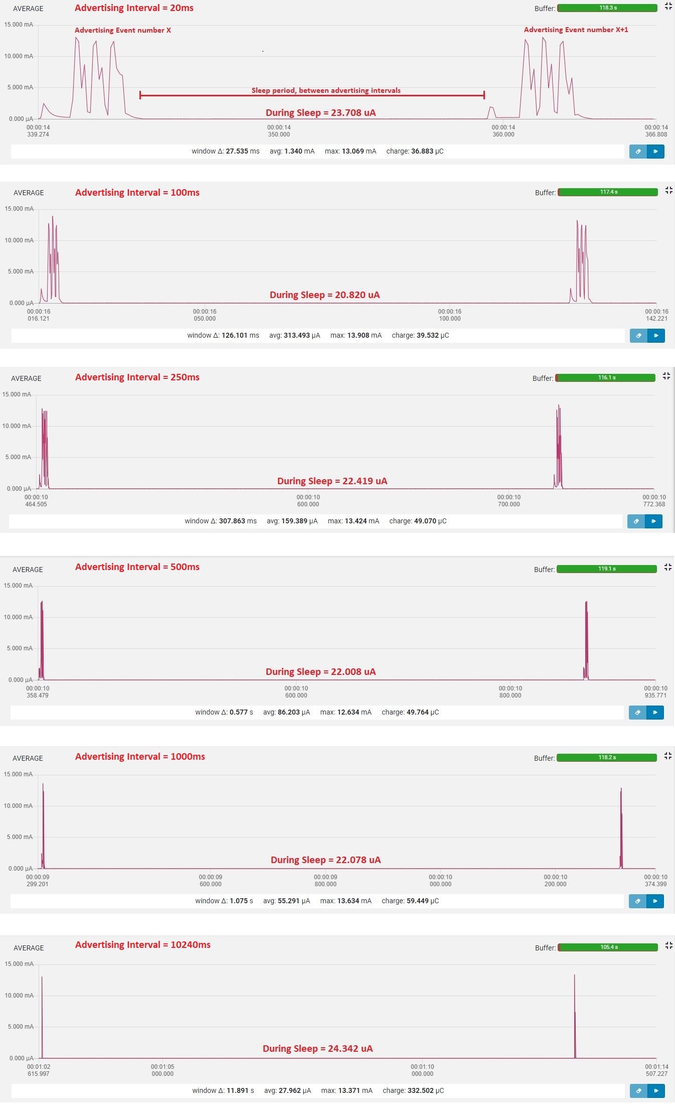
In the above image, each snapshot represents the measured current consumption by the nRF52840 chip at different advertising intervals. The two peaks represent advertising events, the period between them represents current consumption during sleep.
2. Advertising Data Length
It is the length of the payload which is transmitted during the advertising events. During the transmission of the payload, the radio circuitry is on.
Specification limit: 31 bytes
The below image summarizes the measured current consumption for various advertising data length. With an empty payload, the average power consumption was found to be around 1.4 mA and with a full payload of 31 bytes, the average power consumption was found to be around 2.1 mA.
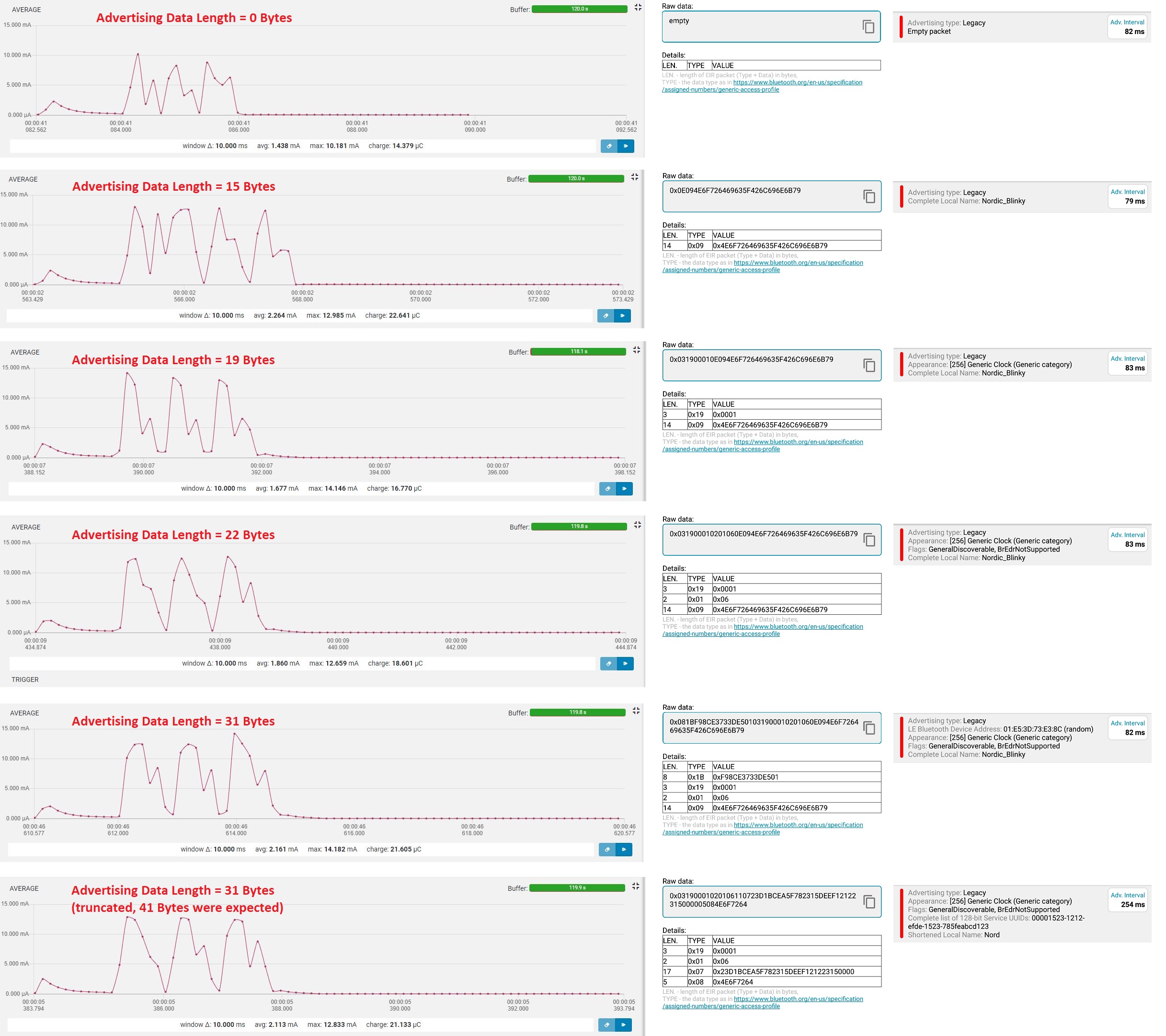
In the above Image, each snapshot represents measured current with corresponding advertising data.
Connection Parameters
1. Connection Interval
It is the time interval between two consecutive connection events. During the connection event, the radio is turned on for data exchange. Shorter connection intervals yield higher throughput. For example, with a connection interval of 100ms, the 10 connection events occur within a period of 1 second. Similar to advertising interval, shorter intervals consume more power than longer intervals.
Specification Limit: 7.5ms to 4s
The table below summarizes the measured current consumption at various connection intervals.
| Connection Interval in ms | Avg. Current in uA | Peak Current in mA |
| 20 | 244.198 | 10.163 |
| 100 | 111.722 | 10.265 |
| 250 | 64.926 | 9.967 |
| 500 | 43.394 | 11.598 |
| 1000 | 37.217 | 12.482 |
| 4000 | 25.406 | 11.589 |
We observe that the Avg. Current consumption drops as we increase the connection interval. It also means that data rate reduces due to less frequent connections events.
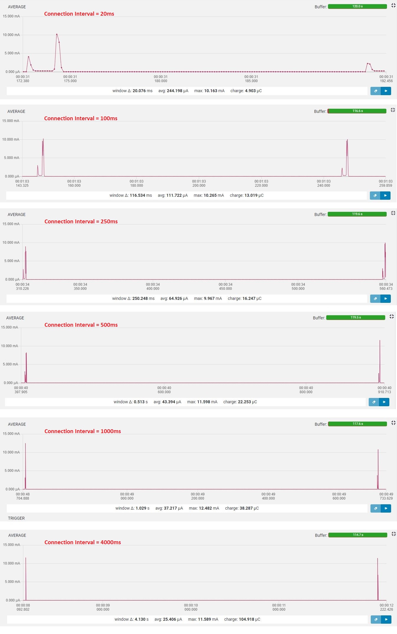
In the above image, each snapshot represents the measured current consumption at different connection intervals. The two peaks represent connection events.
2. Slave Latency
It is the range of a number of connection events that a slave device (peripheral) may skip when it is in an idle state. The device may wake before the next connection event to participate in a BLE transaction if it has something to exchange with the Master/Central device or simply skip it. As an effect, it seems that the sleep period between two connection events expands by the number of skipped connection events.
This relationship helps determine the maximum value of Slave Latency. Supervision_Timeout > (1 + Conn_Latency) * Conn_Interval_Max * 2
For example, with a fixed Connection Interval of 100 ms and Connection Supervision Timeout of 4 seconds, using the relationship above yields slave latency to be lower than 19. This means that a peripheral device is allowed to skip between 0 to 18 connection events. The table below summarizes the measured current consumption within an effective connection interval timeframe due to slave latency.
| Slave Latency in Num. of Conn. Events | Avg. Current in uA | Peak Current in mA |
| 0 | 69.968 | 11.734 |
| 9 | 29.115 | 10.235 |
| 18 | 24.345 | 11.533 |
Compare the avg. current consumption with slave latency of 0 with 9 & 18. The Avg. Current consumption drops with increasing slave latency.
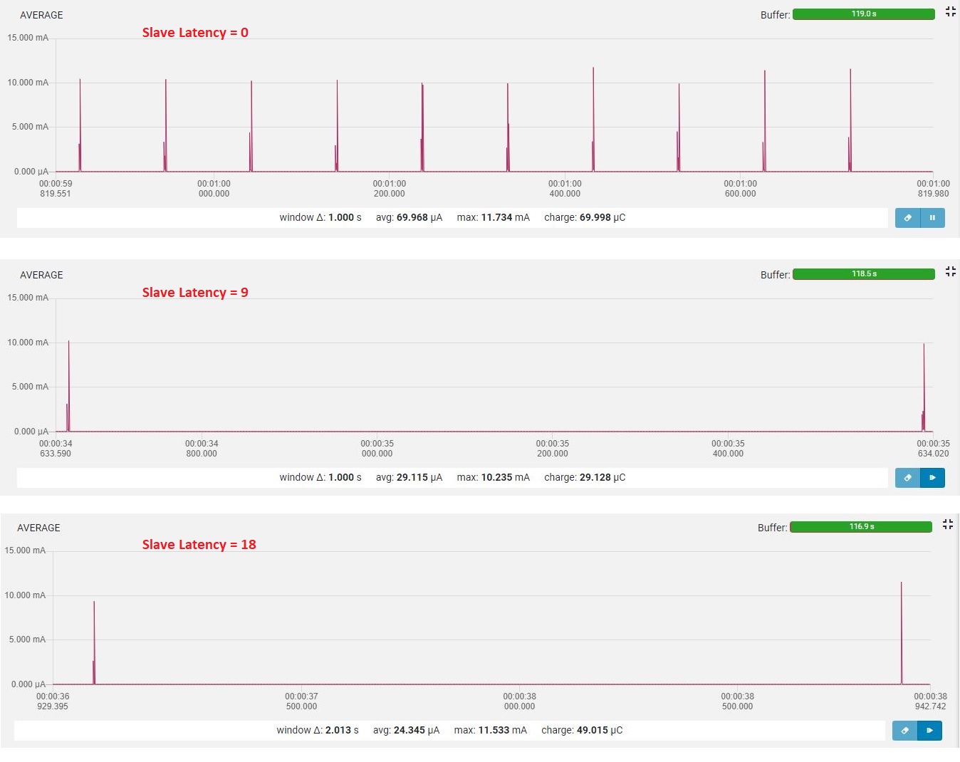 From the above image pay close attention to the time axis and number of peaks, we observe the following:
- At slave latency of 0, the connection events occur periodically at every 100 ms. So in a time-frame of 1 second, we should see 10 connection events at 100 ms intervals.
- At slave latency of 9, the connection events occur periodically by skipping 9 connection events when idle. So in a time-frame of 1 second, we should see around 1 connection event instead of 10 events.
- At slave latency of 18, the connection events occur periodically by skipping 18 connection events when idle. So in a time-frame of 2 seconds, we should see around 2 connection events instead of 20 events.
Radio Parameters
Other than tuning advertising and connection parameters, the transmission power level of the radio directly impacts the power consumption, radio power level and is expressed in dBm unit. The radio power level can be a pre-set to a fixed value or may be dynamically adjusted based on the distance or received signal strength.
All of the previous tests were out at a 0 dBm level.
TX Power Level
The nRF5-SDK provides an API to set the transmission power level for both advertising and connection state. A Peripheral device may host a Transmission Power Service to which a Central device may read or write to adjust the power level of a peripheral device. If the distance between the two devices in connection is fixed & remains immobile then it’s possible to determine and set the optimal power level required when in connection. The table below shows the measured average and peak current consumption at various power levels starting from the highest to the lowest. The connection interval was set to 100ms for this test.
| Tx Radio Power Level | Avg. Current in uA | Peak Current in mA |
| +8 dBm | 140.67 | 25.088 |
| +4 dBm | 110.598 | 17.888 |
| 0 dBm | 121.504 | 11.447 |
| -4 dBm | 105.664 | 9.67 |
| -8 dBm | 106.244 | 12.287 |
| -12 dBm | 101.446 | 11.44 |
| -16 dBm | 99.89 | 11.387 |
| -20 dBm | 99.843 | 11.55 |
| -40 dBm | 99.719 | 12.906 |
We observe that the Avg. Current consumption increases when the radio power level is incremented.
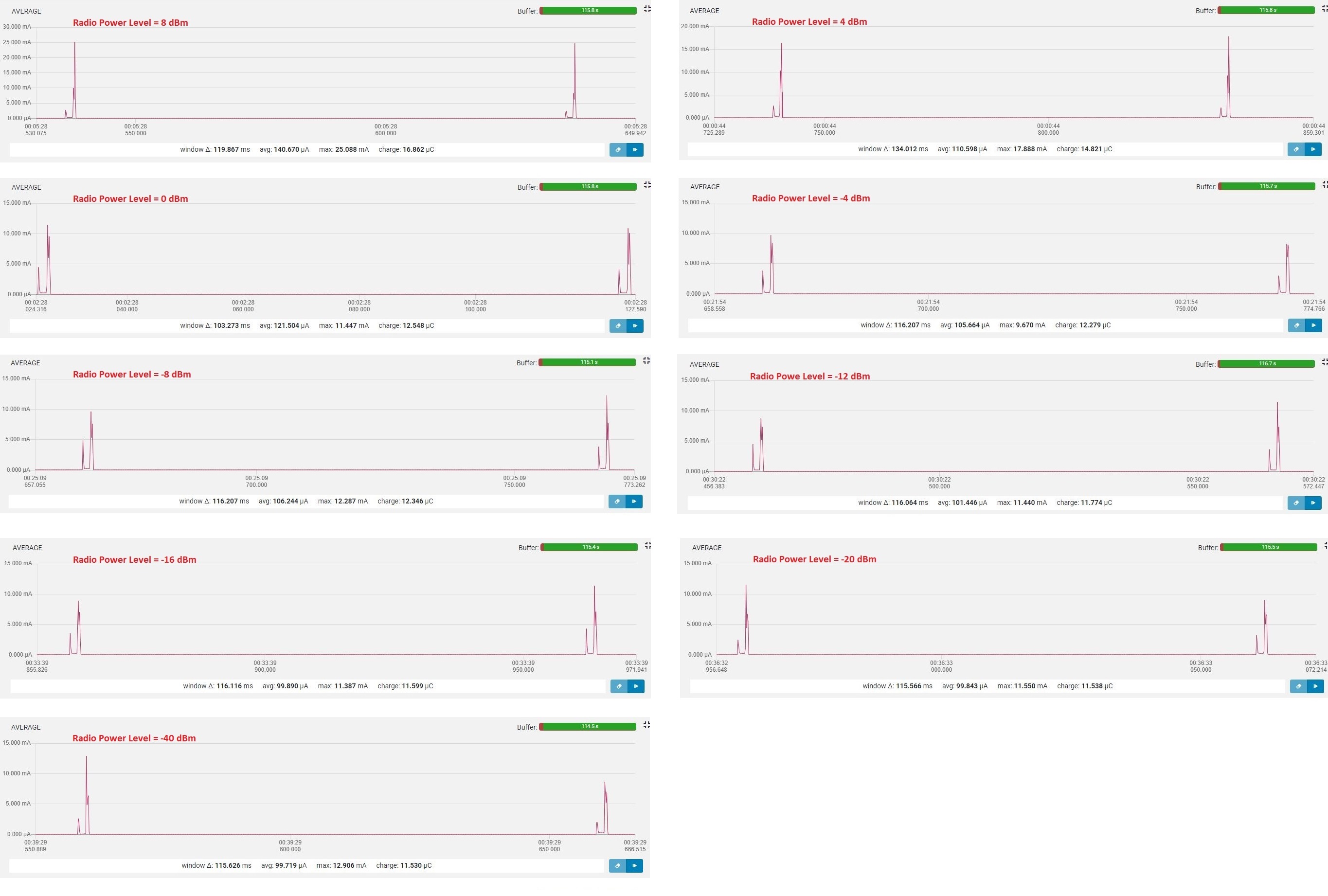
In the above image, each snapshot represents the measured current consumption at different radio levels. The two peaks represent connection events with a connection interval of 100ms.
Summary
Two simple factors that directly affect power consumption are:
- The duration of time for which the radio is on, and
- The power level of the radio.
These factors are dependent on the parameters that we have seen in this post.
- Advertising Parameters: Fast and Slow advertising terms are commonly used for describing advertising rates. For fast advertising the advertising interval is lower, therefore the probability of the device discovery is higher, hence higher power consumption. For slow advertising, the advertising interval is higher, the probability of the device discovery is lower, hence lower power consumption. Advertising beacons utilize complete payload. Connection dependent devices may or may not require to utilize full payload, only necessary information can be advertised.
- Connection Parameters: A peripheral might advertise preferred connection parameters. The central device may establish a connection within the preferred parameters. Not all devices require high throughput, for these devices the connection interval could be higher, hence lower power consumption. For bulk data transfers higher throughput is suitable, therefore lower connection interval is preferred, hence higher power consumption.
- Radio Power Level: The range of communication is dependent on the power level, distance, and line of sight. By tuning the power level one could optimize the required power level based on the signal strength between the devices.